Flux

Thermal and Reflected light modeling tools.

This includes computations such as NEATM, FRM, HG, and reflection models.

Modeling is broken into categories of complexity, ranging from pure black body calculations, through to telescope specific models. Picking the appropriate model can save significant development time, but removes some of the control for the user.

For multi-band thermal + reflected light modeling, use neatm_model_flux() or frm_model_flux(). These evaluate the model in parallel across multiple geometries and return ModelResults objects containing total, thermal, and reflected fluxes.

Use resolve_hg_params() to compute any missing value from the (H-mag, diameter, visible albedo) triad before calling the model functions.

If optical wavelengths are the goal, hg_apparent_mag() or hg_apparent_flux() is probably appropriate.

There are a number of lower-level functions provided more for pedagogical reasons:

lambertian_flux()
frm_facet_temps()
neatm_facet_temps()

class kete.flux.FitResult

Full MCMC fitting result.

beaming: Posterior statistics for beaming (NEATM only). None for FRM/HG. Only non-divergent draws are included.

best_fit_fluxes: Model fluxes at the MAP point for each observation (Jy).

best_fit_reflected_frac: Reflected-light fraction at the MAP point, one per observation.

best_fit_residuals: Standardized residuals (obs - model) / (f_sigma * sigma) at the MAP.

chi2_best: Reduced chi-squared at the MAP point using inflated uncertainties.

columns: Column names for each element of a draw vector.

diameter: Posterior statistics for diameter (km). None for HG model. Only non-divergent draws are included.

divergent: Per-draw divergence flags from the NUTS sampler.

draws: Non-divergent MCMC posterior draws. Each row is one sample; column layout depends on the model (see columns).

draws_all: All MCMC posterior draws including divergent transitions. Use divergent to identify which rows diverged.

f_sigma: Posterior statistics for uncertainty inflation factor. Only non-divergent draws are included.

g_param: Posterior statistics for G parameter. Only non-divergent draws are included.

h_mag: Posterior statistics for H magnitude. Only non-divergent draws are included.

ir_albedo_ratio: Posterior statistics for IR-to-visible albedo ratio. None for HG model. Only non-divergent draws are included.

model: Model name ("Neatm", "Frm", or "Hg").

n_divergent: Total number of divergent transitions.

nobs: Number of non-upper-limit observations.

vis_albedo: Posterior statistics for visual geometric albedo. None for HG model. Only non-divergent draws are included.

class kete.flux.FluxObs(flux, sigma, band, sun2obj, sun2obs, is_upper_limit=False)

A single flux observation at a known geometry.

Parameters:

flux – Observed flux in Jy (or upper-limit threshold).
sigma – 1-sigma uncertainty in Jy.
band – Band identifier: a WISE name ("W1"-"W4") or a wavelength in nm.
sun2obj – Sun-to-object vector in AU (Ecliptic frame).
sun2obs – Sun-to-observer vector in AU (Ecliptic frame).
is_upper_limit – If True, flux is a non-detection upper limit.

flux: Observed flux in Jy.

is_upper_limit: Whether this is a non-detection upper limit.

sigma: 1-sigma uncertainty in Jy.

sun2obj: Sun-to-object vector in AU (Ecliptic frame), as [x, y, z].

sun2obs: Sun-to-observer vector in AU (Ecliptic frame), as [x, y, z].

wavelength: Band wavelength in nm.

class kete.flux.FluxPriors(diameter=None, beaming=None, r_ir=None, h_mag=None, g_param=None, vis_albedo=None)

Priors used in thermal model fitting, below is the list of default priors.

Priors can be specified either using the FluxPriors constructor or by directly passing a tuple of the form (low, high) for bounds-only or (low, high, mean, sigma) for bounds + Gaussian. Below we see the defaults being specified using the tuple form.

Not all of these priors are used in every model, this is a comprehensive list for all models.

If not provided, defaults are used, specifying a prior will overwrite the specified priors while leaving the others at their defaults:

kete.flux.FluxPriors(
    diameter   = (0.001, 1000),
    beaming    = (0.5, 3.0, 1.0, 0.3),
    r_ir       = (0.5, 2.0, 1.6, 0.3),
    h_mag      = (-5.0, 35.0),
    g_param    = (-0.3, 0.7, 0.2, 0.05),
    vis_albedo = (0.01, 1.0),
)

Each prior is a ParamPrior specifying bounds (logistic barrier) and an optional gaussian centering prior (mean, sigma). To effectively fix a parameter, set tight bounds around the desired value (e.g., bounds=(val - 1e-3, val + 1e-3)).

Parameters:

diameter – ParamPrior for diameter D in km.
beaming – ParamPrior for beaming parameter.
r_ir – ParamPrior for IR-to-visible albedo ratio R_IR.
h_mag – ParamPrior for H magnitude.
g_param – ParamPrior for G parameter.
vis_albedo – ParamPrior for visible geometric albedo.

beaming

diameter

g_param

h_mag

r_ir

vis_albedo

class kete.flux.ModelResults(fluxes, thermal_fluxes, hg_fluxes, v_band_magnitude, v_band_flux, magnitudes=None)

Reflected/Thermal model results.

Parameters:

fluxes – Total fluxes per band in units of Jy / Steradian.
thermal_fluxes – Black body specific fluxes per band in units of Jy / Steradian.
hg_fluxes – Reflected light specific fluxes per band in units of Jy / Steradian.
v_band_magnitude – Expected magnitude in the V-band using the HG model.
v_band_flux – Expected flux in the V-band using the HG model.
magnitudes – Magnitudes in the different bands if zero mags were available.

fluxes: Total fluxes per band in units of Jy / Steradian.

hg_fluxes: Reflected light specific fluxes per band in units of Jy / Steradian.

magnitudes: Magnitudes in the different bands if zero mags were available.

thermal_fluxes: Black body specific fluxes per band in units of Jy / Steradian.

v_band_flux: Expected flux in the V-band using the HG model.

v_band_magnitude: Expected magnitude in the V-band using the HG model.

class kete.flux.ParamPrior(bounds, gaussian=None)

Prior configuration for model fitting. Configuration for a single parameter’s prior.

Parameters:

bounds – (low, high) logistic-barrier hard bounds.
gaussian – Optional (mean, sigma) Gaussian centering prior. None means flat (uniform) within the bounds.

bounds

gaussian

kete.flux.black_body_flux(temp, wavelength)

Compute the black body flux at the specified temperatures and wavelength.

Flux is in units Janskys / steradian per unit freq. This can be converted to being per unit wavelength by multiplying the result of this by c / wavelength**2.

This is limited by the size of float 32s, numbers exceeding 1e-300 will be rounded to 0. This should not raise any warnings, and should be relatively numerically stable and correct over most domains of interest.

Parameters:

temp – List of temperatures, in units of Kelvin.
wavelength – In units of nanometers.

Returns:

Janskys per steradian

Return type:

List

kete.flux.bond_albedo(vis_albedo, g_param=0.15)

Approximate the Bond albedo from the visible geometric albedo and the HG slope parameter using Bowell et al. (1989): A_B = vis_albedo * (0.290 + 0.684 * g_param).

For the radiation force model the relevant quantity is the absorptivity alpha = 1 - A_B.

Parameters:

vis_albedo – Visible geometric albedo.
g_param – G phase parameter in the HG system. 0.15 is the typical asteroid default.

kete.flux.comet_apparent_mags(sun2obj, sun2obs, mk_1=None, mk_2=None, phase_corr=Ellipsis)

Given the M1/K1 and M2/K2 values, compute the apparent Comet visible magnitudes.

The model for apparent magnitudes are:

m1 + k1 * log10(sun2obj.r) + 5.0 * log10(obj2obs.r) + phase_mag_slope_1 * phase m2 + k2 * log10(sun2obj.r) + 5.0 * log10(obj2obs.r) + phase_mag_slope_2 * phase

Where m1/k1 are related to total magnitudes and m2/k2 are nucleus magnitudes.

This model is based off of these: https://ssd.jpl.nasa.gov/horizons/manual.html#obsquan (see section 9) https://en.wikipedia.org/wiki/Absolute_magnitude#Cometary_magnitudes

Note that the above model does not include a 2.5x term attached to the K1/2 terms which are present in the wikipedia definition, this matches the definitions used by JPL Horizons.

Note that this includes seperate phase magnitude slope for both the nucleus and total fluxes.

This does a best effort to compute both magnitudes, if any values are missing this will return None in the respective calculation.

Parameters:

sun2obj – A vector-like object containing the X/Y/Z coordinates pointing to the object from the sun in units of AU.
sun2obs – A vector-like object containing the X/Y/Z coordinates pointing from the sun to the observer in units of AU.
mk_1 – Tuple of (M_1, K_1), where M_1 is the total Absolute magnitude of the comet, and K_1 magnitude slope as a function of heliocentric distance.
mk_2 – Tuple of (M_2, K_2), where M_2 is the total Absolute magnitude of the nucleus, and K_2 nucleus magnitude slope as a function of heliocentric distance.
phase_corr – Magnitude variation of the comet as a function of observing phase, units are Mag/Deg of phase, this defaults to 0.0 for the total magnitude, and 0.035 Mag/Deg for the nucleus.

Returns:

(Total apparent magnitude, Magnitude of the nucleus)

Return type:

float

kete.flux.comet_dust_phase_curve_correction(phase_angle)

Phase correction curve for cometary dust from the following paper:

A composite phase function for cometary dust comae Bertini, Ivano, et al. Planetary and Space Science (2025): 106164.

This uses the fitted values from the paper for k=0.80, g_f=0.944, g_b=-0.542.

An additional normalization has been applied so that the value of this is 1.0 at 0.0 phase angle.

Parameters:: phase_angle – The angular separation between the sun and observer as viewed from the dust, units of degrees.
Returns:: The phase curve correction.
Return type:: float

kete.flux.fit_model(model, obs, h_mag=None, g_param=None, emissivity=0.9, priors=None, num_chains=10, num_tune=200, num_draws=500, c_hg=None)

Fit a model to observations using NUTS MCMC.

H magnitude and G parameter are fitted as free parameters. If h_mag or g_param are supplied, they set the center of the corresponding Gaussian prior (keeping its width from priors). emissivity is a fixed thermal property (not fitted).

Parameters:

model – Model name: "neatm", "frm", or "hg".
obs – List of FluxObs observations.
h_mag – Optional H magnitude – sets the center of the H prior.
g_param – Optional G parameter – sets the center of the G prior.
emissivity – Fixed thermal emissivity (default 0.9, not fitted).
priors – Prior configuration (FluxPriors, default if None).
num_chains – Number of MCMC chains (default 10).
num_tune – Warmup draws per chain (default 200).
num_draws – Posterior draws per chain (default 500).
c_hg – HG relationship constant (default 1329.0).

Returns:

MCMC posterior results.

Return type:

FitResult

Raises:

ValueError – If the fit fails to converge.

kete.flux.frm_facet_temps(facet_normals, subsolar_temp, obj2sun)

Calculate the temperatures of each facet assuming the FRM model.

This is a multi-core operation.

Parameters:

facet_normals – List of surface normal vectors.
subsolar_temp – Temperature at the sub-solar point in kelvin.
obj2sun – Vector from the object to the sun in AU.

kete.flux.frm_model_flux(sun2obj, sun2obs, band_albedos, h_mag=None, diameter=None, vis_albedo=None, g_param=0.15, emissivity=0.9, band_wavelengths=None, bands=None, zero_mags=None)

Compute FRM thermal + reflected fluxes for a single geometry.

Evaluates the FRM model for the given Sun-object-observer geometry, computing both thermal emission and reflected solar light (HG model) across multiple wavelength bands simultaneously.

Parameters:

sun2obj – Vector pointing from the Sun to the object (AU).
sun2obs – Vector pointing from the Sun to the observer (AU).
band_albedos – Albedo of the object in each band (0-1).
h_mag – H magnitude of the object in the HG system. At least two of h_mag, diameter, and vis_albedo must be provided.
diameter – Diameter of the object in km.
vis_albedo – Visible geometric albedo.
g_param – G phase coefficient, defaults to 0.15.
emissivity – Emissivity of the object, defaults to 0.9.
band_wavelengths – List of effective wavelengths in nm. Required unless bands is given.
bands – Band preset name: "wise", "neos", "irac", "mips", or "irs_pu". If given, band_wavelengths is ignored and the standard band definitions (including color corrections and zero magnitudes) are used.
zero_mags – Optional list of zero-point magnitudes for each band. Only used when band_wavelengths is provided.

Returns:

Fluxes and magnitudes for the given geometry.

Return type:

ModelResults

kete.flux.hg_apparent_flux(sun2obj, sun2obs, g_param, wavelength, vis_albedo, h_mag=None, diameter=None, c_hg=None)

Calculate the reflected flux from an object using the HG asteroid model.

This assumes that the object is an ideal disk facing the sun and applies the IAU correction curve to the reflected light, returning units of Jy per unit frequency.

This treats the sun as a flat black body disk, which is a good approximation as long as the object is several solar radii away.

Either h_mag or diameter must be provided, but only 1 is strictly required. The other will be computed if not provided.

Parameters:

sun2obj – A vector-like object containing the X/Y/Z coordinates pointing from the sun to the object in units of AU.
sun2obs – A vector-like object containing the X/Y/Z coordinates pointing from the sun to the observer in units of AU.
g_param – The G parameter of the object.
wavelength – The wavelength of the object in nanometers.
vis_albedo – The geometric albedo of the object at the specified wavelength.
h_mag – H magnitude of the object in V band.
diameter – The diameter of the object in km.
c_hg – The relationship constant between H, D, and pV for the bandpass. Defaults to 1329.0.

Returns:

Flux in Jy per unit frequency.

Return type:

float

kete.flux.hg_apparent_mag(sun2obj, sun2obs, h_mag, g_param)

Compute the apparent magnitude of an object using the absolute magnitude H, G, and positional information.

The HG IAU model is not technically defined above 120 degrees phase, however this will continue to return values fit to the model until 160 degrees. Phases larger than 160 degrees will return nan.

Parameters:

sun2obj – A vector-like object containing the X/Y/Z coordinates pointing from the sun to the object in units of AU.
sun2obs – A vector-like object containing the X/Y/Z coordinates pointing from the sun to the observer in units of AU.
G – The G parameter of the object.
H – The absolute magnitude of the object.

Returns:

The apparent magnitude of the object.

Return type:

float

kete.flux.hg_phase_curve_correction(g_param, phase_angle)

This computes the phase curve correction in the IAU format.

Parameters:

g_param – The G parameter of the object.
phase_angle – The angular separation between the sun and observer as viewed from the object, units of degrees.

Returns:

The phase curve correction.

Return type:

float

kete.flux.lambertian_flux(facet_flux, facet_normals, obs2obj, diameter, emissivity)

Calculate the visible flux at the observer assuming a convex faceted object made up of a collection of lambertian surfaces.

Parameters:

facet_flux – Flux from each of the facets in Jy / Steradian per unit freq.
facet_normals – List of surface normal vectors.
obs2obj – Vector from the observer to the object in AU.
diameter – Diameter of the object in km.
emissivity – Emissivity of the lambertian surfaces (between 0 and 1, 0.9 is a good default).

kete.flux.neatm_facet_temps(facet_normals, subsolar_temp, obj2sun)

Calculate the temperatures of each facet assuming the NEATM model.

This is a multi-core operation.

Parameters:

facet_normals – List of surface normal vectors.
subsolar_temp – Temperature at the sub-solar point in kelvin.
obj2sun – Vector from the object to the sun in AU.

kete.flux.neatm_model_flux(sun2obj, sun2obs, band_albedos, h_mag=None, diameter=None, vis_albedo=None, g_param=0.15, beaming=1.0, emissivity=0.9, band_wavelengths=None, bands=None, zero_mags=None)

Compute NEATM thermal + reflected fluxes for a single geometry.

Evaluates the NEATM model for the given Sun-object-observer geometry, computing both thermal emission and reflected solar light (HG model) across multiple wavelength bands simultaneously.

Parameters:

sun2obj – Vector pointing from the Sun to the object (AU).
sun2obs – Vector pointing from the Sun to the observer (AU).
band_albedos – Albedo of the object in each band (0-1).
h_mag – H magnitude of the object in the HG system. At least two of h_mag, diameter, and vis_albedo must be provided.
diameter – Diameter of the object in km.
vis_albedo – Visible geometric albedo.
g_param – G phase coefficient, defaults to 0.15.
beaming – Beaming parameter, defaults to 1.0.
emissivity – Emissivity of the object, defaults to 0.9.
band_wavelengths – List of effective wavelengths in nm. Required unless bands is given.
bands – Band preset name: "wise", "neos", "irac", "mips", or "irs_pu". If given, band_wavelengths is ignored and the standard band definitions (including color corrections and zero magnitudes) are used.
zero_mags – Optional list of zero-point magnitudes for each band. Only used when band_wavelengths is provided.

Returns:

Fluxes and magnitudes for the given geometry.

Return type:

ModelResults

kete.flux.resolve_hg_params(h_mag=None, vis_albedo=None, diameter=None, c_hg=None)

Resolve any two of (h_mag, vis_albedo, diameter) to compute the third.

Given any two of H-magnitude, visible geometric albedo, and diameter, this computes the missing value using the standard C_hg relationship. If all three are provided, it validates that they are consistent.

Parameters:

h_mag – H magnitude of the object in the HG system.
vis_albedo – Visible geometric albedo.
diameter – Diameter of the object in km.
c_hg – The C_hg constant (default 1329.0 km).

Returns:

(h_mag, vis_albedo, diameter) with all three resolved.

Return type:

tuple

kete.flux.solar_flux(dist, wavelength)

Return the Solar flux in Jy / Steradian from the 2000 ASTM Standard Extraterrestrial Spectrum Reference E-490-00: <https://www.nrel.gov/grid/solar-resource/spectra-astm-e490.html>

Returned values are units Janskys / steradian per unit freq.

Parameters:

dist – Distance the object is from the Sun in au.
wavelength – Wavelength in nm.

kete.flux.sub_solar_temperature(sun_dist, vis_albedo, g_param, beaming, emissivity=0.9)

Compute the subsolar surface temperature in kelvin.

Parameters:

sun_dist – Distance from the object to the sun in AU.
vis_albedo – Visible geometric albedo.
g_param – G Phase parameter in the HG system.
beaming – The beaming parameter of the object.
emissivity – Emissivity of the object, 0.9 by default.

shape

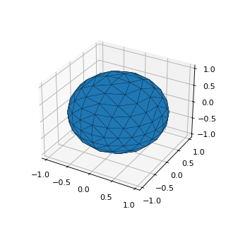
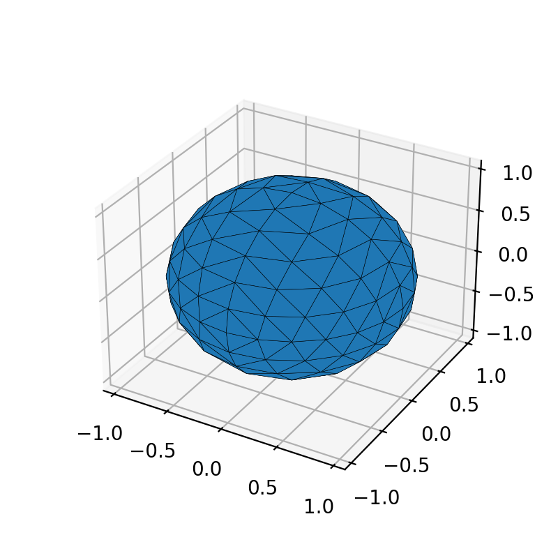
class kete.shape.TriangleEllipsoid(n_div=6, x_scale=1.0, y_scale=1.0, z_scale=1.0)

A triangle-faceted ellipsoid shape, used for visualization of thermal models.

This generates a nearly-uniform triangulation of an ellipsoid using the algorithm from https://arxiv.org/abs/1502.04816.

Examples

(Source code, png, hires.png, pdf)

Parameters:

n_div – Number of divisions from pole to equator. Total facet count is 8 * n_div^2. Must be at least 1.
x_scale – Scale factor along the x-axis.
y_scale – Scale factor along the y-axis.
z_scale – Scale factor along the z-axis.

areas: Area of each facet (normalized so total area is 1), shape (n,).

facets: Triangle vertices of each facet, shape (n, 3, 3).

normals: Unit normal vectors of each facet, shape (n, 3).