2024 YR4 - Orbit Determination from Real Observations
Overview
2024 YR4 is a near-Earth asteroid discovered on 2024 December 27 by the ATLAS survey. Its short initial arc placed it on an elevated-probability impact list for 2032, which generated significant follow-up attention. By early 2025 the impact was ruled out.
This tutorial uses real MPC ADES astrometry to walk through a standard orbit determination:
Fetch optical observations from the Minor Planet Center.
Run Initial Orbit Determination (IOD) to get a starting orbit.
Refine with differential correction and inspect residuals.
Propagate the fitted orbit to the 2032 close-approach epoch.
Note
This tutorial requires network access to the MPC ADES API. Results will
vary as new observations accumulate in the MPC archive. Pass
update_cache=True to fetch_mpc_observations()
to refresh the local cache.
import matplotlib.pyplot as plt
import numpy as np

import kete
1. Fetch Observations
fetch_mpc_observations() queries the MPC web API,
applies the EFCC18 star-catalog debiasing correction, assigns per-observatory
astrometric uncertainties, and returns a list of
Observation objects ready for fitting. Results
are cached locally under ~/.kete/observations/.
obs = kete.orbit_fitting.fetch_mpc_observations("2024 YR4")
print(f"Fetched {len(obs)} observations")

epochs = [o.epoch.jd for o in obs]
arc_days = max(epochs) - min(epochs)
t_start = kete.Time(min(epochs)).iso
t_end   = kete.Time(max(epochs)).iso
print(f"Arc: {t_start[:10]}  to  {t_end[:10]}  ({arc_days:.1f} days)")
Fetched 512 observations
Arc: 2024-12-25  to  2026-02-26  (428.6 days)
2. Initial Orbit Determination
With real observations in hand we run IOD.
initial_orbit_determination() scans a grid of
topocentric distances across observation pairs, solves Lambert’s problem at
each grid point, and scores the candidates by angular residual. Candidates
are returned sorted best-first.
candidates = kete.orbit_fitting.initial_orbit_determination(obs)
print(f"IOD returned {len(candidates)} candidate(s)")

score, best = candidates[0]
elem = best.elements
print(f"Best candidate:  score={score:.3e}")
print(f"  a = {elem.semi_major:.4f} AU")
print(f"  e = {elem.eccentricity:.4f}")
print(f"  i = {elem.inclination:.3f} deg")
IOD returned 3 candidate(s)
Best candidate:  score=2.355e-05
  a = 2.5623 AU
  e = 0.6649
  i = 3.390 deg
3. Differential Correction
fit_orbit() refines the IOD candidate against all
observations. Internally it runs a sequence of windowed least-squares passes
to bootstrap convergence across the full arc, then applies outlier rejection
following the Carpino-Milani-Chesley (2003) algorithm.
fit = kete.orbit_fitting.fit_orbit(best, obs)

print(f"Converged: {fit.converged}")
print(f"RMS:       {fit.rms:.4f}")
included = sum(fit.included)
total    = len(fit.all_observations)
print(f"Included:  {included} / {total} observations")

elem = fit.state.elements
print(f"Fitted elements:")
print(f"  a = {elem.semi_major:.6f} AU")
print(f"  e = {elem.eccentricity:.6f}")
print(f"  i = {elem.inclination:.4f} deg")
print(f"  q = {elem.peri_dist:.6f} AU")
Converged: True
RMS:       0.8633
Included:  479 / 512 observations
Fitted elements:
    a = 2.515890 AU
    e = 0.661415
    i = 3.4082 deg
    q = 0.851843 AU
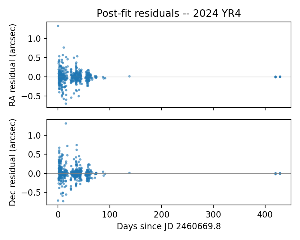
4. Residual Analysis
Post-fit residuals should scatter symmetrically around zero with no clear trend in time. A drift would suggest a force not included in the model.
residuals  = np.array(fit.residuals)
epochs_inc = [o.epoch.jd for o, inc in
              zip(fit.all_observations, fit.included) if inc]
t0 = min(epochs_inc)

fig, (ax1, ax2) = plt.subplots(2, 1, sharex=True, figsize=(5, 4), dpi=200)

ax1.scatter(np.array(epochs_inc) - t0, residuals[:, 0], s=4, alpha=0.5)
ax1.axhline(0, color="gray", lw=0.5)
ax1.set_ylabel("RA residual (arcsec)")
ax1.set_title("Post-fit residuals -- 2024 YR4")

ax2.scatter(np.array(epochs_inc) - t0, residuals[:, 1], s=4, alpha=0.5)
ax2.axhline(0, color="gray", lw=0.5)
ax2.set_ylabel("Dec residual (arcsec)")
ax2.set_xlabel(f"Days since JD {t0:.1f}")

plt.tight_layout()
plt.savefig("data/yr4_residuals.png")
plt.close()
5. Positional Uncertainty vs. JPL Horizons
We compare the spread of sampled orbits from the kete fit against the published JPL Horizons covariance at the 2032 close-approach epoch. Sampling both covariances and propagating forward turns the abstract covariance matrix into a concrete cloud of positions in km. The X-Y and X-Z ecliptic projections show whether the two fits agree in both the size and shape of their uncertainty regions.
First locate the Earth close approach:
earth_now = kete.spice.get_state("Earth", fit.state.jd)
ca_epoch, ca_dist = kete.closest_approach(
    fit.state,
    earth_now,
    kete.Time.from_ymd(2031, 1, 1),
    kete.Time.from_ymd(2033, 1, 1),
)
jd_ca   = ca_epoch.jd
ca_date = kete.Time(jd_ca).iso[:10]
print(f"Closest approach:  {ca_date}  "
      f"({ca_dist * kete.constants.AU_KM:.0f} km, "
      f"{ca_dist:.5f} AU)")
Closest approach: 2032-12-22 (882932 km, 0.00590 AU)
horizons = kete.HorizonsProperties.fetch("2024 YR4")

N_SAMPLES = 200
k_samples, _ = fit.uncertain_state.sample(N_SAMPLES, seed=42)
h_samples, _ = horizons.sample(N_SAMPLES, seed=42)

# Propagate the nominal state and all samples to the close-approach epoch.
k_nom_ca = kete.propagate_n_body(fit.state, jd_ca)
h_nom_ca = kete.propagate_n_body(horizons.state, jd_ca)
k_ca     = kete.propagate_n_body(k_samples, jd_ca)
h_ca     = kete.propagate_n_body(h_samples, jd_ca)

AU_KM = kete.constants.AU_KM

fig, (ax1, ax2) = plt.subplots(2, 1, figsize=(5, 4), dpi=200)

ax1.scatter(
    [(s.pos.x - h_nom_ca.pos.x) * AU_KM for s in h_ca],
    [(s.pos.y - h_nom_ca.pos.y) * AU_KM for s in h_ca],
    c="k", s=4, alpha=0.5, label="JPL Horizons",
)
ax1.scatter(
    [(s.pos.x - k_nom_ca.pos.x) * AU_KM for s in k_ca],
    [(s.pos.y - k_nom_ca.pos.y) * AU_KM for s in k_ca],
    c="tab:red", s=4, alpha=0.5, label="kete",
)
ax1.axhline(0, color="gray", lw=0.4)
ax1.axvline(0, color="gray", lw=0.4)
ax1.set_aspect("equal")
ax1.set_xlabel("Ecliptic X (km)")
ax1.set_ylabel("Ecliptic Y (km)")
ax1.legend(markerscale=3)

ax2.scatter(
    [(s.pos.x - h_nom_ca.pos.x) * AU_KM for s in h_ca],
    [(s.pos.z - h_nom_ca.pos.z) * AU_KM for s in h_ca],
    c="k", s=4, alpha=0.5,
)
ax2.scatter(
    [(s.pos.x - k_nom_ca.pos.x) * AU_KM for s in k_ca],
    [(s.pos.z - k_nom_ca.pos.z) * AU_KM for s in k_ca],
    c="tab:red", s=4, alpha=0.5,
)
ax2.axhline(0, color="gray", lw=0.4)
ax2.axvline(0, color="gray", lw=0.4)
ax2.set_aspect("equal")
ax2.set_xlabel("Ecliptic X (km)")
ax2.set_ylabel("Ecliptic Z (km)")

fig.suptitle("2024 YR4 -- Orbital uncertainty at 2032 close approach\nkete vs. JPL Horizons")
plt.tight_layout()
plt.savefig("data/yr4_uncertainty.png")
plt.close()
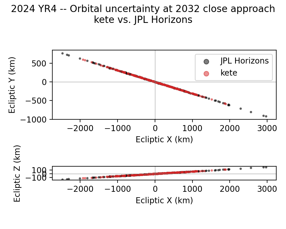
The two clouds overlapping with similar extent indicates the kete fit is consistent with JPL’s in both position and uncertainty. A systematic offset between the cloud centres would point to a difference in the best-fit orbit; a large size mismatch would suggest different observation weighting.
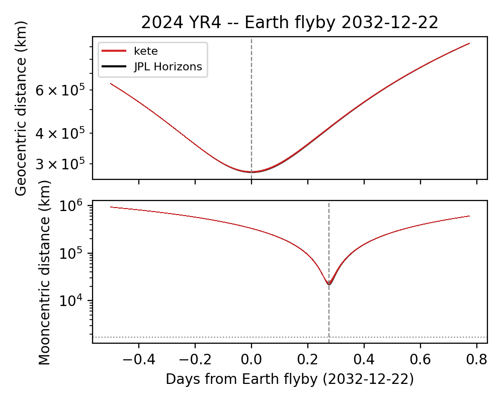
6. Close Approach Distance Envelopes
We find when the nominal orbit passes closest to the Moon, then propagate the full sample cloud across a window that spans both the Earth and Moon flybys. Plotting each sample’s geocentric and selenocentric distance shows the spread of possible miss distances at each event.
# Find the Moon flyby epoch for the nominal orbit.
moon_at_ca    = kete.spice.get_state("Moon", jd_ca)
jd_moon_epoch, moon_dist = kete.closest_approach(
    k_nom_ca,
    moon_at_ca,
    kete.Time(jd_ca - 30),
    kete.Time(jd_ca + 30),
)
jd_moon   = jd_moon_epoch.jd
moon_date = kete.Time(jd_moon).iso[:10]
print(f"Closest approach to Moon: {moon_date}  "
      f"({moon_dist * kete.constants.AU_KM:.0f} km)")
Closest approach to Moon: 2032-12-24 (196832 km)
AU_KM    = kete.constants.AU_KM
jd_start = min(jd_ca, jd_moon) - 0.5
jd_end   = max(jd_ca, jd_moon) + 0.5
jd_steps = np.linspace(jd_start, jd_end, 300)

# At each step propagate all samples in one batch call and record distances.
k_earth = []   # (steps, samples)
h_earth = []
k_moon  = []
h_moon  = []

for jd in jd_steps:
    k_at    = kete.propagate_n_body(k_ca, jd)
    h_at    = kete.propagate_n_body(h_ca, jd)
    moon_pos = kete.spice.get_state("Moon", jd, center=399).pos

    k_earth.append([s.change_center(399).pos.r * AU_KM for s in k_at])
    h_earth.append([s.change_center(399).pos.r * AU_KM for s in h_at])
    k_moon.append(
        [(s.change_center(399).pos - moon_pos).r * AU_KM for s in k_at])
    h_moon.append(
        [(s.change_center(399).pos - moon_pos).r * AU_KM for s in h_at])

k_earth = np.array(k_earth)   # (steps, samples)
h_earth = np.array(h_earth)
k_moon  = np.array(k_moon)
h_moon  = np.array(h_moon)
t       = jd_steps - jd_ca    # days relative to Earth flyby

fig, (ax1, ax2) = plt.subplots(2, 1, sharex=True, figsize=(5, 4), dpi=200)

for ax, k, h, event_jd, label in [
    (ax1, k_earth, h_earth, jd_ca,   "Geocentric distance (km)"),
    (ax2, k_moon,  h_moon,  jd_moon, "Mooncentric distance (km)"),
]:
    for i in range(h.shape[1]):
        ax.plot(t, h[:, i], c="k",       lw=0.3, alpha=0.15)
    for i in range(k.shape[1]):
        ax.plot(t, k[:, i], c="tab:red", lw=0.3, alpha=0.2)
    ax.axvline(event_jd - jd_ca, color="gray", lw=0.8, ls="--")
    ax.set_ylabel(label)
    ax.set_yscale("log")
plt.axhline(kete.constants.MOON_RADIUS_AU * AU_KM, color="gray", lw=0.8, ls=":")

# Legend proxies.
import matplotlib.lines as mlines
ax1.add_artist(mlines.Line2D([], [], color="tab:red", label="kete"))
ax1.add_artist(mlines.Line2D([], [], color="k",       label="JPL Horizons"))
ax1.legend(fontsize=8)
ax1.set_title(f"2024 YR4 -- Earth flyby {ca_date}")
ax2.set_xlabel(f"Days from Earth flyby ({ca_date})")

plt.tight_layout()
plt.savefig("data/yr4_close_approach.png")
plt.close()