NEATM Thermal Fitting with Simulated WISE Data
Overview
This tutorial demonstrates the full workflow of thermal model fitting using the NEATM (Near-Earth Asteroid Thermal Model). We will:
Define a synthetic asteroid with known physical properties.
Construct a realistic orbit and compute observation geometries.
Simulate WISE W1–W4 band flux measurements with noise.
Fit the NEATM model to those observations using MCMC.
Compare the recovered posterior to the true input parameters.
This is the standard workflow for characterizing asteroid diameters and albedos from mid-infrared survey data. We include all four WISE bands: W1 (3.4 um), W2 (4.6 um), W3 (12 um), and W4 (22 um). The shorter wavelength bands carry reflected-light information while W3 and W4 are dominated by thermal emission.
Note
This example takes about a minute to run due to the MCMC sampling step.
1. Define the True Asteroid
We choose physical properties typical of a moderate-albedo S-type main-belt asteroid:
import matplotlib.pyplot as plt
import numpy as np
import kete

np.random.seed(42)

# True physical parameters
# km
true_diam = 10.0
# geometric albedo
true_vis_albedo = 0.15
# NEATM beaming parameter
true_beaming = 1.2
# HG phase parameter
true_g_param = 0.15
# thermal emissivity (fixed, not fitted)
true_emissivity = 0.9
# IR-to-visible albedo ratio
true_r_ir = 1.6

# Derive H magnitude from diameter and albedo
true_h_mag = kete.compute_h_mag(true_diam, true_vis_albedo)
print(f"True parameters:")
print(f"  Diameter:  {true_diam} km")
print(f"  Albedo:    {true_vis_albedo}")
print(f"  H mag:     {true_h_mag:.2f}")
print(f"  Beaming:   {true_beaming}")
print(f"  G param:   {true_g_param}")
print(f"  R_IR:      {true_r_ir}")
True parameters:
  Diameter:  10.0 km
  Albedo:    0.15
  H mag:     12.68
  Beaming:   1.2
  G param:   0.15
  R_IR:      1.6
2. Build an Orbit and Compute Geometries
We construct a main-belt orbit and pick several observation epochs spread across a lunation. At each epoch we compute the Sun-to-object and Sun-to-observer (Earth) vectors, which define the observation geometry.
# Main-belt orbit
epoch = kete.Time.from_ymd(2024, 3, 15)
elements = kete.CometElements(
    desig="TestAsteroid",
    epoch=epoch,
    eccentricity=0.08,
    inclination=10.0,
    peri_arg=75.0,
    lon_of_ascending=45.0,
    peri_time=kete.Time(epoch.jd - 200),
    peri_dist=2.5,
)
state = elements.state
print(f"Orbit: a={elements.semi_major:.3f} AU, "
      f"e={elements.eccentricity:.3f}, "
      f"i={elements.inclination:.1f} deg")
Orbit: a=2.717 AU, e=0.080, i=10.0 deg
Simulate 8 observations spread over 30 days, representing repeated WISE scans of the same field:
obs_jds = epoch.jd + np.array([0, 1, 5, 6, 14, 15, 29, 30])
print(f"Observing over {obs_jds[-1] - obs_jds[0]:.0f} day arc")

geometries = []
for jd in obs_jds:
    obj_state = kete.propagate_two_body(state, jd)
    earth = kete.spice.get_state("Earth", jd)
    sun2obj = obj_state.pos
    sun2obs = earth.pos
    geometries.append((sun2obj, sun2obs))

# Print example geometry
sun2obj_0, sun2obs_0 = geometries[0]
helio_dist = sun2obj_0.r
geo_dist = (sun2obj_0 - sun2obs_0).r
print(f"First epoch:  r_helio={helio_dist:.3f} AU, "
      f"r_geo={geo_dist:.3f} AU")
Observing over 30 day arc
First epoch:  r_helio=2.570 AU, r_geo=1.594 AU
3. Simulate WISE Observations
We use neatm_model_flux() to compute the true thermal
+ reflected flux in all four WISE bands, then add Gaussian noise to
simulate real measurements.
ir_albedo = true_r_ir * true_vis_albedo
band_names = ["W1", "W2", "W3", "W4"]

# Evaluate the model at each geometry
model_outputs = [
    kete.flux.neatm_model_flux(
        sun2obj, sun2obs,
        band_albedos=[ir_albedo] * 4,
        h_mag=true_h_mag,
        vis_albedo=true_vis_albedo,
        diameter=true_diam,
        beaming=true_beaming,
        g_param=true_g_param,
        emissivity=true_emissivity,
        bands="wise",
    )
    for sun2obj, sun2obs in geometries
]

# Extract true fluxes for all four bands
true_fluxes = {}
for idx, name in enumerate(band_names):
    true_fluxes[name] = [out.fluxes[idx] for out in model_outputs]

for name in band_names:
    print(f"True {name} fluxes (Jy): "
          f"{[f'{f:.4f}' for f in true_fluxes[name]]}")
Now add 5% Gaussian noise to create the observed fluxes, and package
them as FluxObs objects:
# 5% flux uncertainty
sigma_frac = 0.05
observations = []

for i, (sun2obj, sun2obs) in enumerate(geometries):
    for name in band_names:
        true_flux = true_fluxes[name][i]
        sigma = sigma_frac * true_flux
        noisy_flux = true_flux + np.random.normal(0, sigma)
        obs = kete.flux.FluxObs(
            flux=noisy_flux,
            sigma=sigma,
            band=name,
            sun2obj=sun2obj,
            sun2obs=sun2obs,
        )
        observations.append(obs)

n_bands = len(band_names)
print(f"Created {len(observations)} FluxObs "
      f"({len(observations) // n_bands} epochs x {n_bands} bands)")
True W1 fluxes (Jy): ['0.0007', '0.0007', '0.0006', '0.0006', '0.0006', '0.0005', '0.0004', '0.0004']
True W2 fluxes (Jy): ['0.0008', '0.0008', '0.0008', '0.0008', '0.0007', '0.0007', '0.0006', '0.0006']
True W3 fluxes (Jy): ['0.0838', '0.0836', '0.0823', '0.0818', '0.0776', '0.0770', '0.0668', '0.0660']
True W4 fluxes (Jy): ['0.2212', '0.2206', '0.2173', '0.2163', '0.2058', '0.2042', '0.1780', '0.1760']
Created 32 FluxObs (8 epochs x 4 bands)
4. Run MCMC Fitting
We call fit_model() with model="neatm".
Passing h_mag as a convenience argument centers the H-magnitude
prior on our approximate value (in a real scenario this would come
from optical-survey photometry).
The fitter explores 6 parameters:
[D, beaming, H, G, f_sigma, R_IR]
and returns posterior draws in physical units.
result = kete.flux.fit_model(
    model="neatm",
    obs=observations,
    h_mag=true_h_mag,
    g_param=true_g_param,
    emissivity=true_emissivity,
    num_chains=4,
    num_tune=200,
    num_draws=500,
)

print(f"MCMC complete: {len(result.draws)} draws, "
      f"{result.n_divergent} divergent")
print(f"reduced chi2 = {result.chi2_best:.2f} "
      f"(nobs = {result.nobs}, dof = {result.nobs - 6})")
print(f"\nPosterior summary:")
print(f"  Diameter:  {result.diameter}")
print(f"  Albedo:    {result.vis_albedo}")
print(f"  Beaming:   {result.beaming}")
print(f"  H mag:     {result.h_mag}")
print(f"  G param:   {result.g_param}")
print(f"  R_IR:      {result.ir_albedo_ratio}")
MCMC complete: 2000 draws, 0 divergent
reduced chi2 = 1.27 (nobs = 32, dof = 26)

Posterior summary:
Diameter:  SampleStats(median=9.9621, std=0.1297, ci=[9.7316, 10.2383])
Albedo:    SampleStats(median=0.1511, std=0.0229, ci=[0.1213, 0.2066])
Beaming:   SampleStats(median=1.2035, std=0.0237, ci=[1.1569, 1.2505])
H mag:     SampleStats(median=12.6745, std=0.1496, ci=[12.3363, 12.9049])
G param:   SampleStats(median=0.1368, std=0.0388, ci=[0.0662, 0.2169])
R_IR:      SampleStats(median=1.6059, std=0.2071, ci=[1.1802, 1.9611])
5. Visualize the Posterior
We plot histograms of the key fitted parameters with the true values
overlaid. The NEATM draw columns are
[diameter, vis_albedo, beaming, h_mag, g_param, ir_albedo_ratio, f_sigma].
draws = np.array(result.draws)
columns = result.columns
true_vals = {
    "diameter": true_diam,
    "vis_albedo": true_vis_albedo,
    "beaming": true_beaming,
    "h_mag": true_h_mag,
    "g_param": true_g_param,
    "ir_albedo_ratio": true_r_ir,
}
labels = {
    "diameter": "Diameter (km)",
    "vis_albedo": r"Geometric Albedo $p_V$",
    "beaming": "Beaming",
    "h_mag": "H magnitude",
    "g_param": "G parameter",
    "ir_albedo_ratio": r"$R_{IR}$",
}

fig, axes = plt.subplots(2, 3, figsize=(12, 7))
fig.suptitle("NEATM Posterior -- Simulated WISE W1-W4")

for ax, col_name in zip(axes.flat, labels):
    idx = columns.index(col_name)
    vals = draws[:, idx]
    ax.hist(vals, bins=30, density=True, alpha=0.5, color="steelblue")
    ax.axvline(true_vals[col_name], color="red", ls="--",
               lw=1.5, label="Truth")
    ax.set_xlabel(labels[col_name])
    ax.legend(fontsize=8)

plt.tight_layout()
plt.savefig("data/neatm_fit_posterior.png", dpi=120)
plt.close()
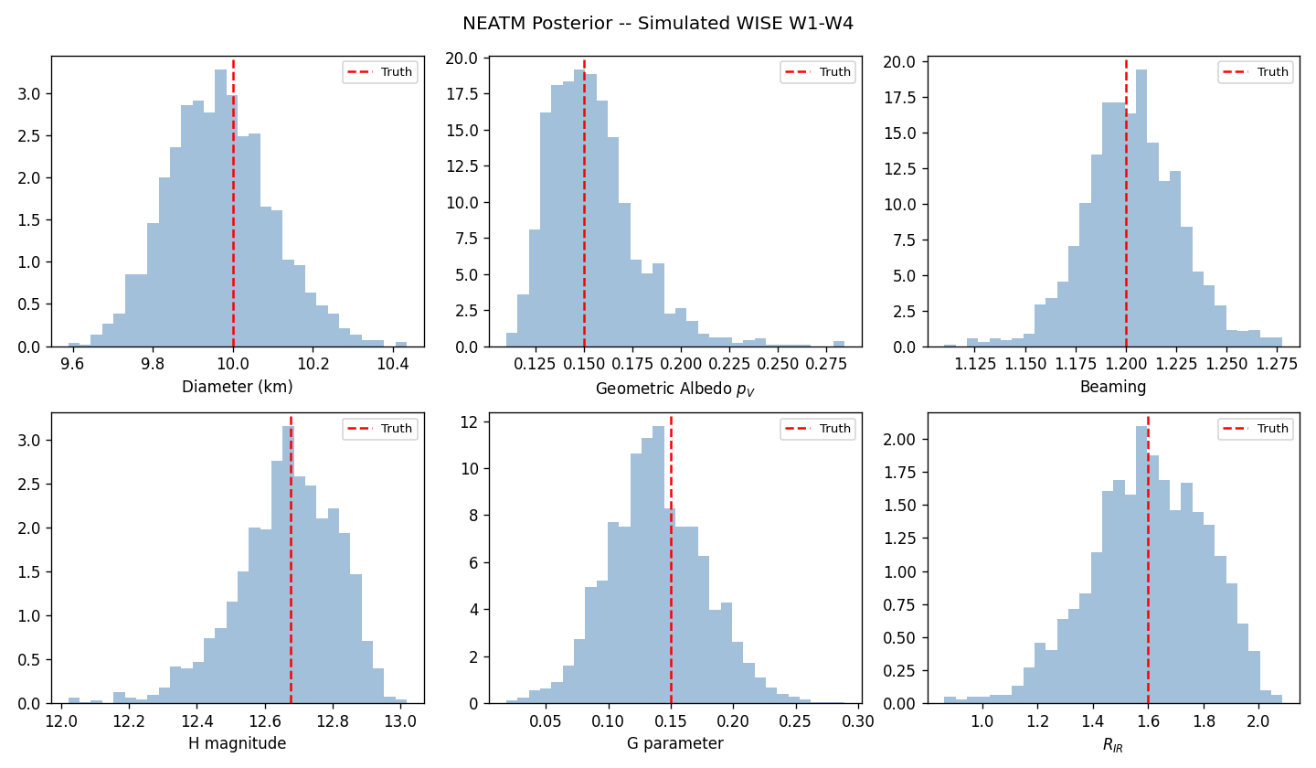
The posterior distributions should be centered near the true values (red dashed lines), confirming that the MCMC sampler successfully recovers the input parameters from noisy thermal data.
6. Diameter–Albedo Degeneracy
A hallmark of thermal fitting is the strong anti-correlation between diameter and albedo: a smaller, brighter asteroid can produce the same thermal flux as a larger, darker one. We visualize this by plotting the joint posterior:
d_idx = columns.index("diameter")
pv_idx = columns.index("vis_albedo")

fig, ax = plt.subplots(figsize=(6, 5))
ax.scatter(draws[:, d_idx], draws[:, pv_idx],
           s=2, alpha=0.3, color="steelblue")
ax.scatter(true_diam, true_vis_albedo,
           c="red", s=80, marker="*", zorder=5, label="Truth")
ax.set_xlabel("Diameter (km)")
ax.set_ylabel(r"Geometric Albedo $p_V$")
ax.set_title(r"Diameter vs. Albedo ($D^2 \cdot p_V$ degeneracy)")
ax.legend()
plt.tight_layout()
plt.savefig("data/neatm_fit_diam_albedo.png", dpi=120)
plt.close()
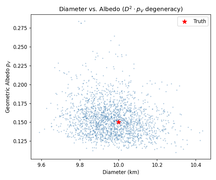
The banana-shaped scatter reflects the constraint imposed by H magnitude: \(D = C_{HG} / \sqrt{p_V} \times 10^{-H/5}\). Every draw lies on the curve defined by the fitted H; the spread along the curve is determined by the thermal data.
7. Residuals and Model Fit Quality
The MAP (maximum a posteriori) fit provides best-fit fluxes and normalized residuals for each observation. Well-behaved residuals should scatter around zero with unit variance.
residuals = np.array(result.best_fit_residuals)
fit_fluxes = np.array(result.best_fit_fluxes)
obs_fluxes = np.array([o.flux for o in observations])

# Group observation indices by band
band_idx = {name: list(range(k, len(observations), n_bands))
            for k, name in enumerate(band_names)}
markers = {"W1": "D", "W2": "^", "W3": "o", "W4": "s"}
colors = {"W1": "C0", "W2": "C1", "W3": "C2", "W4": "C3"}

fig, axes = plt.subplots(1, 2, figsize=(10, 4))

ax = axes[0]
for name in band_names:
    idx = band_idx[name]
    ax.errorbar(range(len(idx)), obs_fluxes[idx],
                yerr=[observations[i].sigma for i in idx],
                fmt=markers[name], ms=4, label=f"{name} obs",
                color=colors[name])
    ax.plot(range(len(idx)), fit_fluxes[idx], "x",
            ms=6, color=colors[name], label=f"{name} model")
ax.set_xlabel("Epoch index")
ax.set_ylabel("Flux (Jy)")
ax.set_title("Observed vs. MAP Model Fluxes")
ax.legend(fontsize=7, ncol=2)

ax = axes[1]
ax.bar(range(len(residuals)), residuals, color="steelblue", alpha=0.6)
ax.axhline(0, color="black", lw=0.5)
ax.axhline(1, color="gray", ls="--", lw=0.5)
ax.axhline(-1, color="gray", ls="--", lw=0.5)
ax.set_xlabel("Observation index")
ax.set_ylabel("Normalized residual")
ax.set_title(f"MAP Residuals ($\\chi^2_\\nu$ = {result.chi2_best:.2f}, "
             f"nobs = {result.nobs})")
plt.tight_layout()
plt.savefig("data/neatm_fit_residuals.png", dpi=120)
plt.close()
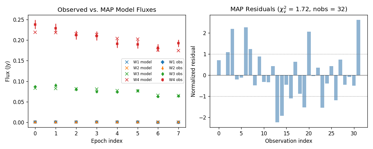
Residuals within \(\pm 1\) indicate a good fit. A reduced \(\chi^2_\nu\) near 1.0 indicates the model explains the data at the level of the measurement noise.
8. Customizing Priors
The default priors work well for most cases, but they can be customized
via FluxPriors and ParamPrior.
For example, to tighten the beaming prior around 1.0:
custom_priors = kete.flux.FluxPriors(
    beaming=kete.flux.ParamPrior(
        bounds=(0.5, 3.0),
        # tighter sigma
        gaussian=(1.0, 0.1),
    ),
)
result_custom = kete.flux.fit_model(
    model="neatm",
    obs=observations,
    h_mag=true_h_mag,
    g_param=true_g_param,
    priors=custom_priors,
    num_chains=4,
    num_tune=200,
    num_draws=500,
)
print(f"Default beaming: {result.beaming}")
print(f"Custom  beaming: {result_custom.beaming}")
Default beaming: SampleStats(median=1.2048, std=0.0221, ci=[1.1618, 1.2513])
Custom  beaming: SampleStats(median=1.1971, std=0.0214, ci=[1.1559, 1.2436])
The tighter prior narrows the posterior, which can be useful when external information constrains the beaming parameter.
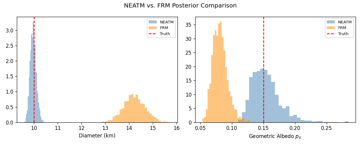
9. NEATM vs. FRM: Model Mismatch
The FRM (Fast Rotating Model) assumes the asteroid rotates fast enough that surface temperature is uniform at each latitude. This is physically different from NEATM, which concentrates thermal emission on the sub-solar hemisphere with an adjustable beaming parameter.
Since our synthetic data were generated with NEATM (beaming = 1.2), fitting with FRM should produce a poorer fit: the wrong thermal distribution will force the fitter to compensate by shifting diameter and albedo.
result_frm = kete.flux.fit_model(
    model="frm",
    obs=observations,
    h_mag=true_h_mag,
    g_param=true_g_param,
    emissivity=true_emissivity,
    num_chains=4,
    num_tune=200,
    num_draws=500,
)

print("FRM posterior summary:")
print(f"  Diameter:  {result_frm.diameter}")
print(f"  Albedo:    {result_frm.vis_albedo}")
print(f"  H mag:     {result_frm.h_mag}")
print(f"  R_IR:      {result_frm.ir_albedo_ratio}")
print(f"  reduced chi2: {result_frm.chi2_best:.2f} "
      f"(nobs = {result_frm.nobs}, dof = {result_frm.nobs - 5})")
print(f"\nNEATM reduced chi2: {result.chi2_best:.2f}")
print(f"FRM  reduced chi2:  {result_frm.chi2_best:.2f}")
FRM posterior summary:
  Diameter:  SampleStats(median=14.1470, std=0.4187, ci=[13.3563, 14.9973])
  Albedo:    SampleStats(median=0.0749, std=0.0045, ci=[0.0666, 0.0842])
  H mag:     SampleStats(median=12.6776, std=0.0099, ci=[12.6579, 12.6967])
  R_IR:      SampleStats(median=1.7725, std=0.1077, ci=[1.5556, 1.9778])
  reduced chi2: 2.13 (nobs = 32, dof = 27)

NEATM reduced chi2: 1.27
FRM  reduced chi2:  2.13
Compare the diameter and albedo posteriors side by side:
draws_frm = np.array(result_frm.draws)
columns_frm = result_frm.columns

fig, axes = plt.subplots(1, 2, figsize=(10, 4))

for ax, col_name, label, true_val in [
    (axes[0], "diameter", "Diameter (km)", true_diam),
    (axes[1], "vis_albedo", r"Geometric Albedo $p_V$", true_vis_albedo),
]:
    neatm_vals = draws[:, columns.index(col_name)]
    frm_vals = draws_frm[:, columns_frm.index(col_name)]
    ax.hist(neatm_vals, bins=30, density=True, alpha=0.5,
            color="steelblue", label="NEATM")
    ax.hist(frm_vals, bins=30, density=True, alpha=0.5,
            color="darkorange", label="FRM")
    ax.axvline(true_val, color="red", ls="--", lw=1.5, label="Truth")
    ax.set_xlabel(label)
    ax.legend(fontsize=8)

fig.suptitle("NEATM vs. FRM Posterior Comparison")
plt.tight_layout()
plt.savefig("data/neatm_vs_frm_posterior.png", dpi=120)
plt.close()
Now compare the residuals from both models:
residuals_frm = np.array(result_frm.best_fit_residuals)

fig, axes = plt.subplots(1, 2, figsize=(10, 4), sharey=True)

ax = axes[0]
ax.bar(range(len(residuals)), residuals, color="steelblue", alpha=0.6)
ax.axhline(0, color="black", lw=0.5)
ax.axhline(1, color="gray", ls="--", lw=0.5)
ax.axhline(-1, color="gray", ls="--", lw=0.5)
ax.set_xlabel("Observation index")
ax.set_ylabel("Normalized residual")
ax.set_title(f"NEATM ($\\chi^2_\\nu$ = {result.chi2_best:.2f})")

ax = axes[1]
ax.bar(range(len(residuals_frm)), residuals_frm, color="darkorange", alpha=0.6)
ax.axhline(0, color="black", lw=0.5)
ax.axhline(1, color="gray", ls="--", lw=0.5)
ax.axhline(-1, color="gray", ls="--", lw=0.5)
ax.set_xlabel("Observation index")
ax.set_title(f"FRM ($\\chi^2_\\nu$ = {result_frm.chi2_best:.2f})")

fig.suptitle("Residual Comparison: NEATM vs. FRM")
plt.tight_layout()
plt.savefig("data/neatm_vs_frm_residuals.png", dpi=120)
plt.close()
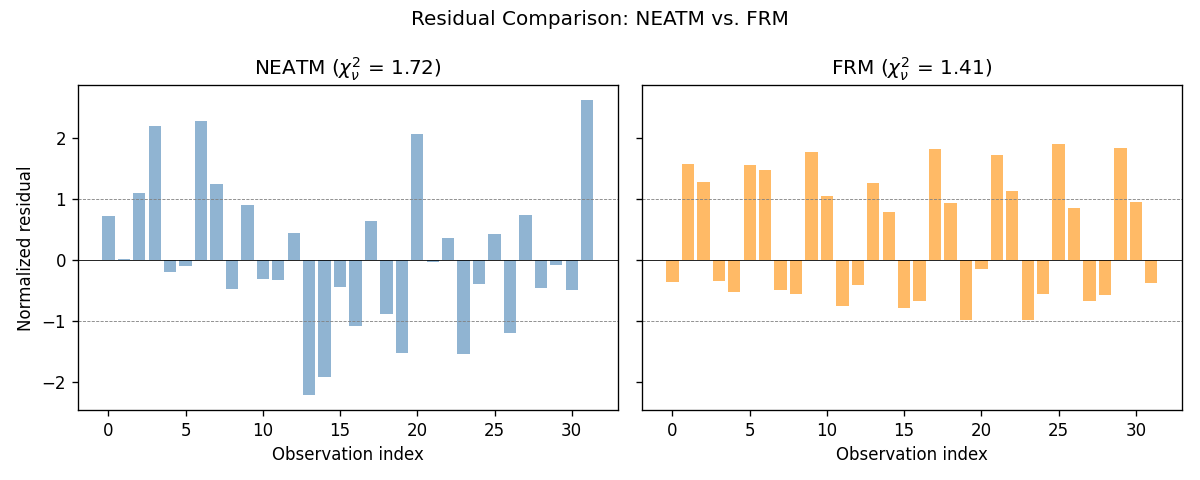
The FRM fit shows larger residuals and a higher \(\chi^2\) because the assumed thermal distribution does not match the data. The diameter and albedo posteriors are shifted away from the true values as the model compensates for the wrong temperature profile. This illustrates why model selection matters: when beaming departs from \(\pi\), NEATM provides a better description of the thermal emission than FRM.