B-Plane Projection

When one body approaches another on a hyperbolic trajectory, it follows a curved path that far from the encounter asymptotes to a line. The incoming asymptote is the straight-line path the body would follow if there were no gravity.

The B-plane is the plane that passes through the center of the target body and is perpendicular to this incoming asymptote. Imagine looking down the barrel of the incoming trajectory: the B-plane is the target you see, with the target body at the origin.

The B-vector points from the center of the target body to the point where the incoming asymptote pierces this plane. Its length is the impact parameter – the distance by which the body would miss if there were no gravity. A larger B-vector means a wider miss; a B-vector of zero means a head-on collision.

The B-plane is split into two axes:

• B dot T: component along the intersection of the B-plane with the ecliptic.

• B dot R: component perpendicular to T within the B-plane.

Together these give a 2D coordinate for the encounter geometry.

This example demonstrates B-plane computation using the 2029 close approach of Apophis to Earth.

import matplotlib.pyplot as plt
import numpy as np

import kete

Fetch Apophis and find the close approach

We fetch the orbit of Apophis from JPL Horizons, then use N-body propagation to find the epoch of closest approach to Earth. The B-plane is evaluated at this epoch.

obj = kete.HorizonsProperties.fetch("Apophis")

# Get Earth's state at the object's epoch to use as the second body
earth = kete.spice.get_state("Earth", obj.state.jd)

# Find the closest approach epoch within a 20-year window
jd_start = obj.state.jd
jd_end = jd_start + 365.25 * 20
ca_time, ca_dist = kete.closest_approach(obj.state, earth, jd_start, jd_end)

print(f"Closest approach: {ca_time.iso}")
print(f"Distance: {ca_dist * kete.constants.AU_KM:.0f} km")

Closest approach: 2029-04-13T21:45:03.631+00:00
Distance: 38011 km

Nominal B-plane

Propagate the nominal orbit to the close approach epoch, re-center on Earth, and compute the B-plane.

state_ca = kete.propagate_n_body(obj.state, ca_time.jd, non_gravs=[obj.non_grav])
geo_state = state_ca.change_center(399)

bp = kete.compute_b_plane(geo_state)

print("B-Plane parameters:")
print(f"  B dot T:          {bp.b_t * kete.constants.AU_KM:12.1f} km")
print(f"  B dot R:          {bp.b_r * kete.constants.AU_KM:12.1f} km")
print(f"  |B|:              {bp.b_mag * kete.constants.AU_KM:12.1f} km")
print(f"  theta:            {np.degrees(bp.theta):12.2f} deg")
print(f"  v_inf:            {bp.v_inf * kete.constants.AU_KM / 86400:12.3f} km/s")
print(f"  Closest approach: {bp.closest_approach * kete.constants.AU_KM:12.1f} km")

B-Plane parameters:
  B dot T:               38962.0 km
  B dot R:               28546.8 km
  |B|:                   48300.7 km
  theta:                   36.23 deg
  v_inf:                   5.841 km/s
  Closest approach:      38011.5 km

Orbital uncertainty in the B-plane

A key use of the B-plane is understanding how orbital uncertainty maps onto encounter geometry. We sample the full covariance matrix of the orbit, propagate each sample to the encounter epoch with N-body mechanics, and plot where each lands in the B-plane.

This type of analysis is commonly used in planetary defense to visualize how orbital uncertainty translates into encounter geometry.

n_samples = 200
states, non_gravs = obj.sample(n_samples)
earth_radius_km = 6371

# Propagate all samples to the close approach epoch
propagated = kete.propagate_n_body(states, ca_time.jd, non_gravs=non_gravs)

b_t_vals = []
b_r_vals = []
n_impacts = 0
for st in propagated:
    geo = st.change_center(399)
    try:
        bp_sample = kete.compute_b_plane(geo)
        bt = bp_sample.b_t * kete.constants.AU_KM
        br = bp_sample.b_r * kete.constants.AU_KM
        if not (np.isfinite(bt) and np.isfinite(br)):
            # NaN B-plane likely means a grazing/impact trajectory
            n_impacts += 1
        elif bp_sample.b_mag * kete.constants.AU_KM < earth_radius_km:
            n_impacts += 1
        else:
            b_t_vals.append(bt)
            b_r_vals.append(br)
    except ValueError:
        # Non-hyperbolic w.r.t. Earth -- count as an impact
        n_impacts += 1

if n_impacts > 0:
    print(
        f"Impact trajectories: {n_impacts} / {n_samples} samples ({100 * n_impacts / n_samples:.1f}%)"
    )

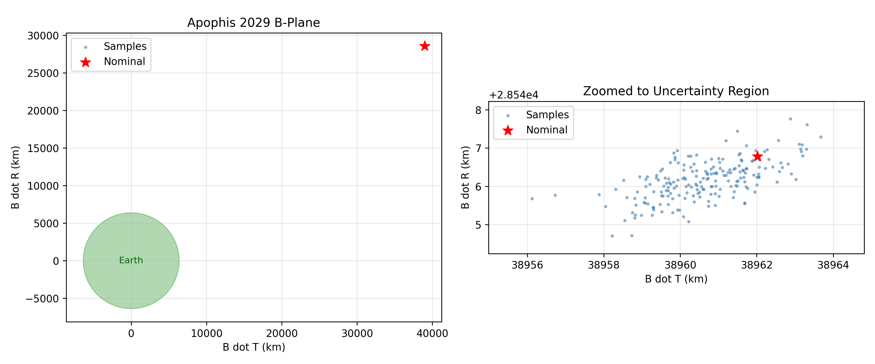
Visualize the B-plane

The nominal encounter point and the cloud of sampled encounters. The spread shows how the current orbital uncertainty maps onto the B-plane.

b_t_arr = np.array(b_t_vals)
b_r_arr = np.array(b_r_vals)

nom_bt = bp.b_t * kete.constants.AU_KM
nom_br = bp.b_r * kete.constants.AU_KM

fig, (ax1, ax2) = plt.subplots(1, 2, figsize=(12, 5), dpi=250)

# Left panel: full view with Earth for scale
for ax in (ax1, ax2):
    ax.scatter(b_t_arr, b_r_arr, s=5, c="steelblue", alpha=0.5, label="Samples")
    ax.scatter(nom_bt, nom_br, s=100, c="red", marker="*", zorder=5, label="Nominal")
    ax.set_xlabel("B dot T (km)")
    ax.set_ylabel("B dot R (km)")
    ax.set_aspect("equal")
    ax.legend()
    ax.grid(True, alpha=0.3)

earth_circle = plt.Circle((0, 0), earth_radius_km, color="green", alpha=0.3)
ax1.add_patch(earth_circle)
ax1.annotate("Earth", (0, 0), ha="center", va="center", fontsize=9, color="darkgreen")
ax1.set_title("Apophis 2029 B-Plane")

# Right panel: zoomed to the sampled region
if len(b_t_arr) > 1:
    margin = 0.15
    span_t = b_t_arr.max() - b_t_arr.min()
    span_r = b_r_arr.max() - b_r_arr.min()
    ax2.set_xlim(b_t_arr.min() - margin * span_t, b_t_arr.max() + margin * span_t)
    ax2.set_ylim(b_r_arr.min() - margin * span_r, b_r_arr.max() + margin * span_r)
ax2.set_title("Zoomed to Uncertainty Region")

plt.tight_layout()
plt.show()