Orbit Fitting from Scratch

Observe Ceres 10 times over six months using SPICE ephemerides, then recover the orbit from scratch using initial orbit determination (IOD) and batch least-squares differential correction.

This demonstrates the full workflow of the kete.fitting module:

1. Generate synthetic optical observations from an Earth-based observer.

2. Run IOD to get a preliminary orbit.

3. Refine with differential correction.

4. Compare the fitted orbit to the SPICE truth.

import matplotlib.pyplot as plt
import numpy as np

import kete

Generate Synthetic Observations

We observe Ceres from Palomar Mountain (MPC code 675) at 10 epochs spread evenly over six months. We use OmniDirectionalFOV and fov_state_check which apply proper light-time correction automatically.

jd_start = kete.Time.from_ymd(2025, 1, 1).jd
jd_end = kete.Time.from_ymd(2025, 7, 1).jd
jd_obs = np.linspace(jd_start, jd_end, 10)

# Get the true Ceres state at the first epoch (Sun-centered, the default).
ceres_state = kete.spice.get_state("Ceres", jd_obs[0])

# Build one omnidirectional FOV per epoch, observed from Palomar (675).
# The default center is the Sun, matching the Ceres state above.
fovs = []
for jd in jd_obs:
    observer = kete.spice.mpc_code_to_ecliptic("675", jd)
    fovs.append(kete.OmniDirectionalFOV(observer))

# Check visibility -- this propagates Ceres to each epoch with light-time.
visible = kete.fov_state_check([ceres_state], fovs)

# Convert each detection to a fitting Observation.
# The fitting module expects SSB-centered equatorial observers.
observations = []
for vis in visible:
    observer = vis.fov.observer.as_equatorial.change_center(0)
    ra, dec, _, _ = vis.ra_dec_with_rates[0]

    obs = kete.fitting.Observation.optical(
        observer=observer,
        ra=ra,
        dec=dec,
        sigma_ra=0.1 / max(np.cos(np.radians(dec)), 1e-6),
        sigma_dec=0.1,
    )
    observations.append(obs)

print(
    f"Generated {len(observations)} observations spanning {jd_end - jd_start:.0f} days"
)
for i, obs in enumerate(observations):
    print(f"  [{i}] JD {obs.epoch.jd:.2f}  RA={obs.ra:.4f}  Dec={obs.dec:.4f}")

Generated 10 observations spanning 181 days
  [0] JD 2460676.50  RA=313.1109  Dec=-24.8487
  [1] JD 2460696.61  RA=321.1384  Dec=-22.6703
  [2] JD 2460716.72  RA=329.1192  Dec=-20.2410
  [3] JD 2460736.83  RA=336.9327  Dec=-17.6560
  [4] JD 2460756.95  RA=344.4923  Dec=-15.0251
  [5] JD 2460777.06  RA=351.7265  Dec=-12.4658
  [6] JD 2460797.17  RA=358.5545  Dec=-10.1027
  [7] JD 2460817.28  RA=4.8652  Dec=-8.0671
  [8] JD 2460837.39  RA=10.4947  Dec=-6.4958
  [9] JD 2460857.50  RA=15.1942  Dec=-5.5312

Initial Orbit Determination

candidates = kete.fitting.initial_orbit_determination(observations)
print(f"\nIOD returned {len(candidates)} candidate(s)")

# Pick the lowest eccentricity
best = min(candidates, key=lambda s: s.elements.eccentricity)
print(
    f"Best IOD candidate: a={best.elements.semi_major:.4f} AU, "
    f"e={best.elements.eccentricity:.4f}, "
    f"i={best.elements.inclination:.2f} deg"
)

IOD returned 1 candidate(s)
Best IOD candidate: a=3.6304 AU, e=0.1448, i=10.65 deg

Differential Correction

Refine the IOD solution using all 10 observations.

fit = kete.fitting.fit_orbit(best, observations)
print(f"\nFit converged: RMS = {fit.rms:.4e}")
print(f"Fitted state epoch: JD {fit.state.jd:.6f}")

fitted_elem = fit.state.elements
print(
    f"Fitted elements:  a={fitted_elem.semi_major:.6f} AU, "
    f"e={fitted_elem.eccentricity:.6f}, "
    f"i={fitted_elem.inclination:.4f} deg"
)

# Compare to SPICE truth at the same epoch (Sun-centered Ecliptic, matching fit.state)
truth = kete.spice.get_state("Ceres", fit.state.jd)
truth_elem = truth.elements
print(
    f"SPICE truth:      a={truth_elem.semi_major:.6f} AU, "
    f"e={truth_elem.eccentricity:.6f}, "
    f"i={truth_elem.inclination:.4f} deg"
)

da = abs(fitted_elem.semi_major - truth_elem.semi_major)
de = abs(fitted_elem.eccentricity - truth_elem.eccentricity)
di = abs(fitted_elem.inclination - truth_elem.inclination)
print(f"Differences:      da={da:.2e} AU, de={de:.2e}, di={di:.2e} deg")

Fit converged: RMS = 1.1664e-03
Fitted state epoch: JD 2460857.500801
Fitted elements:  a=2.765954 AU, e=0.079440, i=10.5878 deg
SPICE truth:      a=2.765954 AU, e=0.079440, i=10.5878 deg
Differences:      da=1.65e-07 AU, de=8.30e-08, di=4.16e-07 deg

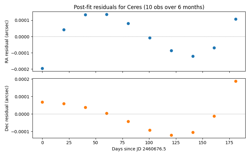
Residuals

Plot the post-fit residuals in RA and Dec.

residuals = np.array(fit.residuals)
epochs = [obs.epoch.jd for obs in observations]
t0 = epochs[0]

fig, (ax1, ax2) = plt.subplots(2, 1, sharex=True, figsize=(8, 5))

# The residuals getter already returns arcseconds for optical observations.
ax1.scatter(np.array(epochs) - t0, residuals[:, 0], c="tab:blue")
ax1.axhline(0, color="gray", ls="--", lw=0.5)
ax1.set_ylabel("RA residual (arcsec)")
ax1.set_title("Post-fit residuals for Ceres (10 obs over 6 months)")

ax2.scatter(np.array(epochs) - t0, residuals[:, 1], c="tab:orange")
ax2.axhline(0, color="gray", ls="--", lw=0.5)
ax2.set_ylabel("Dec residual (arcsec)")
ax2.set_xlabel(f"Days since JD {t0:.1f}")

plt.tight_layout()
plt.show()