Systematic Ranging of a Short-Arc NEO

Demonstrate orbit uncertainty sampling from a single short-arc tracklet using the systematic ranging algorithm (Farnocchia, Chesley & Micheli 2015).

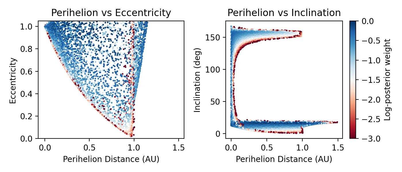
With only a few minutes of observations the orbit is highly degenerate: almost any distance from Earth is consistent with the data. Ranging scans a 2-D grid over topocentric range and range-rate, scores each cell by how well the implied orbit fits the observed curvature, and returns a weighted sample of plausible orbits. The resulting cloud shows the full family of solutions.

import matplotlib.pyplot as plt
import numpy as np

import kete

Parse MPC-Format Observations

Four detections of CEKWD72 from G96 (Catalina Sky Survey, Mt. Lemmon) in standard 80-column MPC format, spanning about 7 minutes on 2026-04-25.

mpc_lines = [
    "     CEKWD72*1C2026 04 25.47779021 00 57.820-00 54 14.76         22.05GVNEOCPG96",
    "     CEKWD72 1C2026 04 25.48209121 00 59.058-00 54 05.11         21.40GVNEOCPG96",
    "     CEKWD72 1C2026 04 25.48639821 01 00.239-00 53 56.47         20.50GVNEOCPG96",
    "     CEKWD72 1C2026 04 25.49071521 01 01.470-00 53 49.27         20.12GVNEOCPG96",
]

mpc_obs = kete.orbit_fitting.MPCObservation.from_lines(mpc_lines)
observations = kete.orbit_fitting.mpc_obs_to_observations(mpc_obs)
print(
    f"Parsed {len(observations)} observations spanning "
    f"{(observations[-1].epoch.jd - observations[0].epoch.jd) * 24 * 60:.1f} minutes"
)

Parsed 4 observations spanning 18.6 minutes

Ranging

Scan the (rho, rho_dot) grid and draw weighted orbit samples.

samples = kete.orbit_fitting.fit_orbit_ranging(observations, num_draws=10000)
print(samples)
if samples.convergence_warning:
    print(f"Warning: {samples.convergence_warning}")

RangingSamples(draws=10000, ess=13513.7, epoch=2461155.978591)

Extract Orbital Elements

draws returns Sun-centered Ecliptic states; each state carries orbital element accessors. We also grab the log-posterior weights for coloring.

states = samples.draws
log_w = np.array(samples.log_posterior)

peri_dist = np.array([s.peri_dist for s in states])
eccentricity = np.array([s.eccentricity for s in states])
inclination = np.array([s.inclination for s in states])

print(f"\nPerihelion distance: {peri_dist.min():.3f} -- {peri_dist.max():.3f} AU")
print(f"Eccentricity:        {eccentricity.min():.3f} -- {eccentricity.max():.3f}")
print(f"Inclination:         {inclination.min():.1f} -- {inclination.max():.1f} deg")

Perihelion distance: 0.000 -- 1.488 AU
Eccentricity:        0.020 -- 4.589
Inclination:         0.3 -- 167.4 deg

Plot the Orbital Uncertainty Cloud

Each point is one sampled orbit, colored by log-posterior weight. The spread shows the full range of solutions consistent with the short arc.

fig, (ax1, ax2) = plt.subplots(1, 2, figsize=(7, 3), dpi=200)

sc = ax1.scatter(
    peri_dist, eccentricity, s=1, c=log_w, cmap="RdBu", vmin=-3, vmax=0, rasterized=True
)
ax1.set_xlabel("Perihelion Distance (AU)")
ax1.set_ylabel("Eccentricity")
ax1.set_title("Perihelion vs Eccentricity")
ax1.set_ylim(0, 1.05)

ax2.scatter(
    peri_dist, inclination, s=1, c=log_w, cmap="RdBu", vmin=-3, vmax=0, rasterized=True
)
ax2.set_xlabel("Perihelion Distance (AU)")
ax2.set_ylabel("Inclination (deg)")
ax2.set_title("Perihelion vs Inclination")

fig.colorbar(sc, ax=ax2, label="Log-posterior weight")
plt.tight_layout()
plt.show()