State Transition Matrix

The State Transition Matrix (STM) describes how a small change in an object’s initial state (position and velocity) maps to a change in its state at a later time:

\[\delta \mathbf{x}(t_f) \approx \Phi(t_f, t_0) \, \delta \mathbf{x}(t_0)\]

This is the foundation of linear orbit determination: rather than re-integrating the orbit for every trial initial condition, a single STM integration gives a first-order approximation valid for small perturbations.

kete computes the STM using the Radau 15th-order integrator with full N-body physics (all planets, GR, J2 oblateness). For objects with non-gravitational forces (comets, dust), extra columns give the partial derivatives of the final state with respect to the non-grav parameters, enabling simultaneous fitting of the orbit and the force model.

This example shows:

1. Computing the 6x6 STM for a simple asteroid orbit.

2. Using the STM to propagate an orbital covariance matrix.

3. Visualizing the 1-sigma position uncertainty ellipse over time.

import matplotlib.pyplot as plt
import numpy as np

import kete

Define an initial state and covariance

We use Ceres as a convenient real object with a well-known orbit, then assign a synthetic diagonal covariance to give it ~10 km position and ~1 m/s velocity uncertainty (expressed in AU and AU/day).

jd_start = kete.Time.j2000().jd
state = kete.spice.get_state("Ceres", jd_start)

# 1-sigma uncertainties
sigma_pos_au = 10 / 1.496e8  # 10 km in AU
sigma_vel_auday = 1 / 1.731e6  # 1 m/s in AU/day

cov0 = np.diag([sigma_pos_au**2] * 3 + [sigma_vel_auday**2] * 3)

Propagate covariance over 1 year

Rather than re-propagating from the initial state at each time step, we chain each integration: the state and covariance from step N become the inputs to step N+1. The covariance update at each step is:

\[P(t_{k+1}) = \Phi_k \, P(t_k) \, \Phi_k^T\]

n_steps = 60
step_days = 365.0 / n_steps
cur_state = state
cur_cov = cov0
pos_sigma_au = [np.sqrt(np.trace(cur_cov[:3, :3]))]
time_steps = [0.0]

for k in range(n_steps):
    jd_next = cur_state.jd + step_days
    cur_state, stm = kete.state_transition.compute_stm(cur_state, jd_next)
    cur_cov = stm @ cur_cov @ stm.T
    pos_sigma_au.append(np.sqrt(np.trace(cur_cov[:3, :3])))
    time_steps.append((k + 1) * step_days)

pos_sigma_km = np.array(pos_sigma_au) * 1.496e8

Inspect the STM at 30 days

compute_stm returns the propagated state and the full 6x6 sensitivity matrix. The STM must be symplectic (det ~= 1) for conservative dynamics.

jd_30 = jd_start + 30
final_state, stm = kete.state_transition.compute_stm(state, jd_30)

print(f"STM determinant at 30 days: {np.linalg.det(stm):.8f}  (should be ~1.0)")
print(f"Final state: {final_state}")

STM determinant at 30 days: 1.00000000  (should be ~1.0)
Final state: State(desig="ceres", jd=2451575.0, pos=[-2.467541144091866, 0.47238990295848526, 0.4692916232900171], vel=[-0.0022900074001403485, -0.01092475456908372, 8.488499757221876e-5], frame=Ecliptic, center="sun")

Sensitivity matrix with a non-gravitational model

For a comet-like object, we can fit A1 (radial), A2 (transverse), and A3 (normal) non-grav parameters simultaneously with the orbit. The STM returns a 6x9 matrix: the first 6 columns are the standard STM, the last 3 are d(final state)/d(A1, A2, A3).

ng_model = kete.propagation.NonGravModel.new_comet(
    a1=1e-9,  # AU/day^2 (typical weak cometary force)
    a2=3e-10,
    a3=0.0,
)

_, sens = kete.state_transition.compute_stm(state, jd_30, non_grav=ng_model)
print(f"\nSensitivity matrix shape with JplComet model: {sens.shape}  (expected: 6x9)")
print("Position sensitivity to A1 at 30 days (AU per AU/day^2):", sens[:3, 6])

Sensitivity matrix shape with JplComet model: (6, 9)  (expected: 6x9)
Position sensitivity to A1 at 30 days (AU per AU/day^2): [-6.37638895  1.18048605  1.8537434 ]

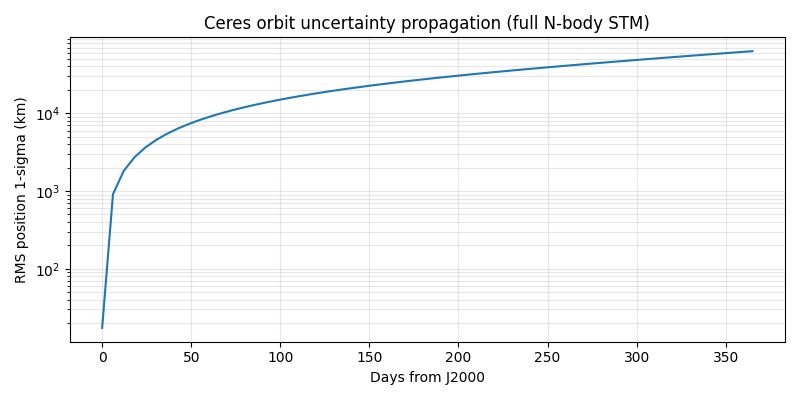
Plot position uncertainty over time

fig, ax = plt.subplots(figsize=(8, 4))
ax.plot(time_steps, pos_sigma_km)
ax.set_xlabel("Days from J2000")
ax.set_ylabel("RMS position 1-sigma (km)")
ax.set_title("Ceres orbit uncertainty propagation (full N-body STM)")
ax.set_yscale("log")
ax.grid(True, which="both", alpha=0.3)
plt.tight_layout()
plt.show()