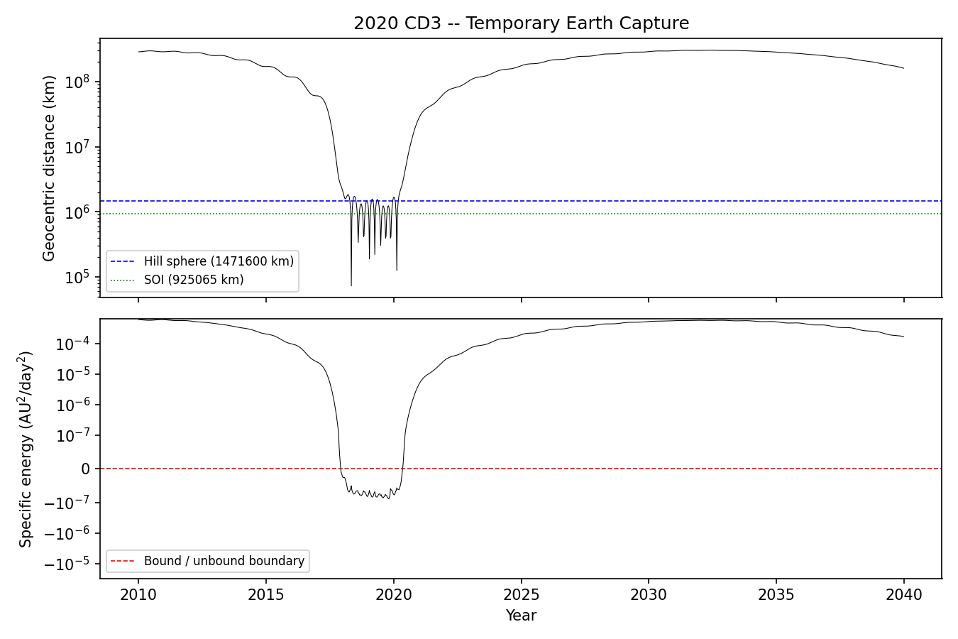
Temporary Earth Capture

Some near-Earth asteroids pass close enough to Earth that they become temporarily captured, orbiting the planet for weeks or months before escaping back onto heliocentric orbits. These so-called “mini-moons” spend time inside Earth’s Hill sphere and can have geocentric specific energy that dips below zero during capture.

This example uses 2020 CD3 – the second known natural object to be temporarily captured by Earth – to demonstrate kete’s orbital analysis tools: geocentric specific energy and Earth’s Hill sphere / sphere of influence.

import matplotlib.pyplot as plt
import numpy as np

import kete

Fetch 2020 CD3 and set up the time window

We fetch the orbit from JPL Horizons and define a window covering the temporary capture event (~Aug 2020 to ~Mar 2021).

obj = kete.HorizonsProperties.fetch("2020 CD3")

jd_start = kete.Time.from_ymd(2010, 1, 1).jd
jd_end = kete.Time.from_ymd(2040, 1, 1).jd

# Propagate to the start of the window
state = kete.propagate_n_body(obj.state, jd_start)

Physical constants

Earth’s Hill sphere and sphere of influence.

planet = "Earth"

earth_hill = kete.hill_radius(planet)
earth_soi = kete.sphere_of_influence(planet)

print(f"Earth Hill radius:     {earth_hill * kete.constants.AU_KM:.0f} km")
print(f"Earth sphere of influence: {earth_soi * kete.constants.AU_KM:.0f} km")

Earth Hill radius:     1471600 km
Earth sphere of influence: 925065 km

Propagate through the capture event

Step through the time window recording geocentric distance and specific energy at each epoch.

step = 7.0  # days
times = np.arange(jd_start, jd_end, step)

geo_dist_km = []
spec_energy = []

for jd in times:
    state = kete.propagate_n_body(state, jd)

    # Geocentric state for distance and specific energy
    geo_state = state.change_center(planet)
    r_km = geo_state.pos.r * kete.constants.AU_KM
    geo_dist_km.append(r_km)

    energy = kete.specific_energy(geo_state)
    spec_energy.append(energy)


geo_dist_km = np.array(geo_dist_km)
spec_energy = np.array(spec_energy)

# Convert JD to fractional year for the x-axis
t_years = [kete.Time(jd).year_float for jd in times]

Plot the results

Two panels show the capture event:

• Geocentric distance relative to Earth’s Hill sphere and sphere of influence.

• Geocentric specific energy – negative values indicate a bound orbit around Earth.

fig, axes = plt.subplots(2, 1, figsize=(9, 6), sharex=True, dpi=150)

ax = axes[0]
ax.plot(t_years, geo_dist_km, "k-", lw=0.5)
ax.axhline(
    earth_hill * kete.constants.AU_KM,
    color="blue",
    ls="--",
    lw=0.8,
    label=f"Hill sphere ({earth_hill * kete.constants.AU_KM:.0f} km)",
)
ax.axhline(
    earth_soi * kete.constants.AU_KM,
    color="green",
    ls=":",
    lw=0.8,
    label=f"SOI ({earth_soi * kete.constants.AU_KM:.0f} km)",
)
ax.set_ylabel("Geocentric distance (km)")
ax.set_yscale("log")
ax.legend(fontsize=8)
ax.set_title(f"{obj.desig} -- Temporary Earth Capture")

ax = axes[1]
ax.plot(t_years, spec_energy, "k-", lw=0.5)
ax.axhline(0, color="red", ls="--", lw=0.8, label="Bound / unbound boundary")
ax.set_ylabel("Specific energy (AU$^2$/day$^2$)")
ax.set_xlabel("Year")
thresh = 10 ** (np.ceil(np.log10(np.abs(np.min(spec_energy)))))
ax.set_yscale("symlog", linthresh=thresh)
ax.legend(fontsize=8)

plt.tight_layout()
plt.show()